library("TSP")dist_mat <-dist(df, diag =TRUE, upper =TRUE)atsp <-as.ATSP(dist_mat)tour <-solve_TSP(atsp)tour#> object of class 'TOUR' #> result of method 'arbitrary_insertion+two_opt' for 10 cities#> tour length: 10.5101
Is this a statistical transformation or a graphical operation?
An aside: Stat vs Geom implementations
Stats are used for transformations1 of data
Geoms are used for converting data structures into their visual representations2
An aside: Stat vs Geom implementations
Things to consider when deciding which to implement:
Can you implement a Stat which “plugs in” to an existing Geom? (e.g. StatSalesperson and GeomSegment)?
Would a user rather have the ability to specify an alternate Stat or Geom?
Which is easier? (typically, the Stat implementation)
Do you need both?
Why extend?
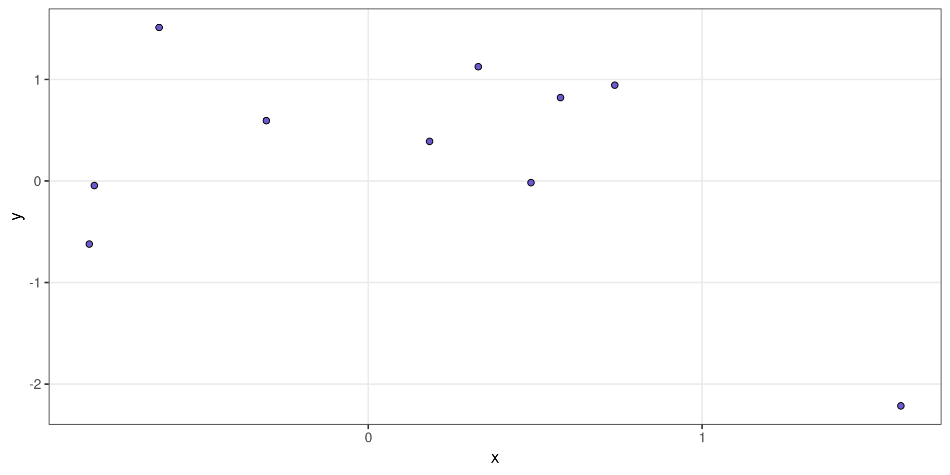
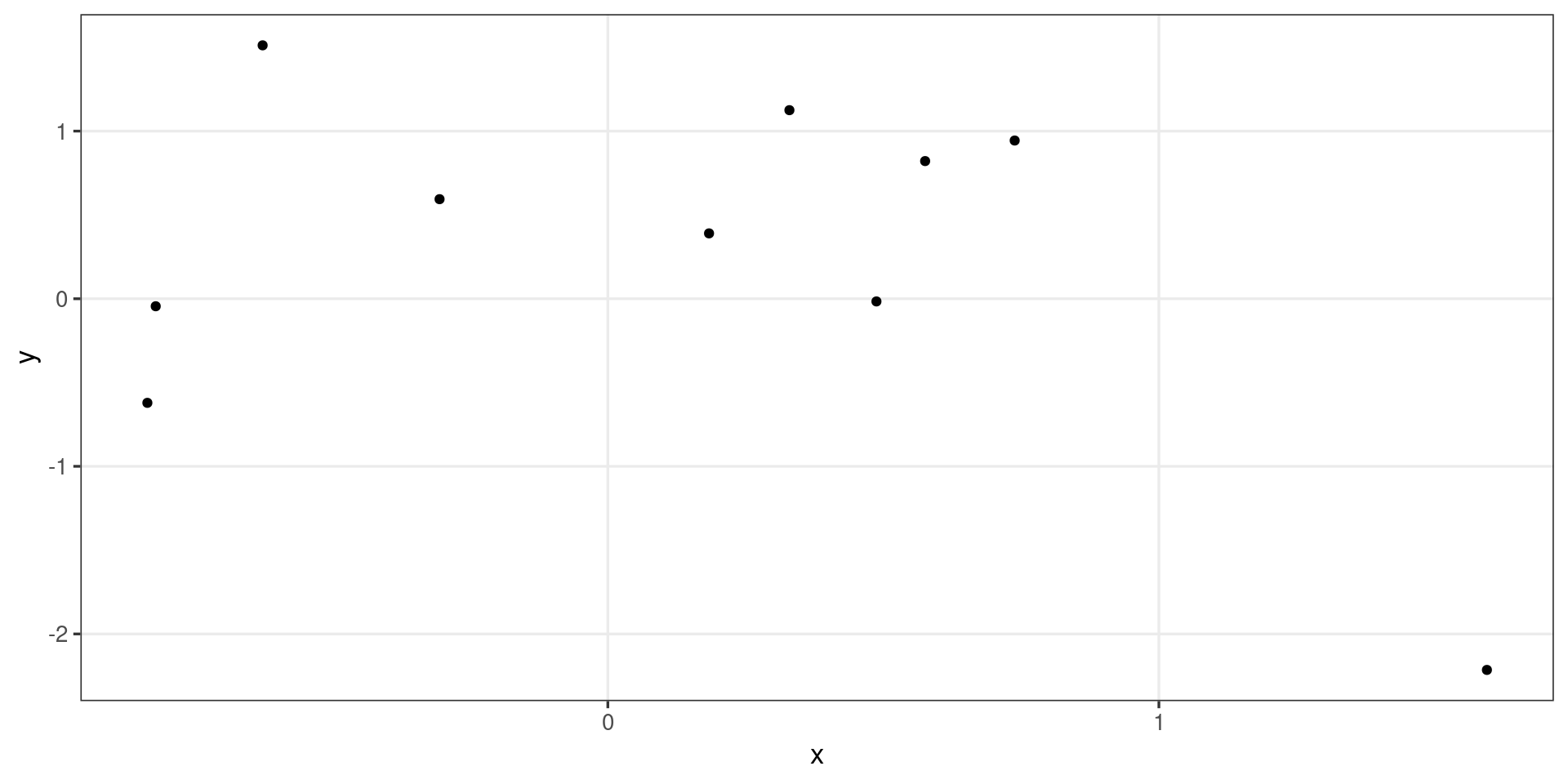
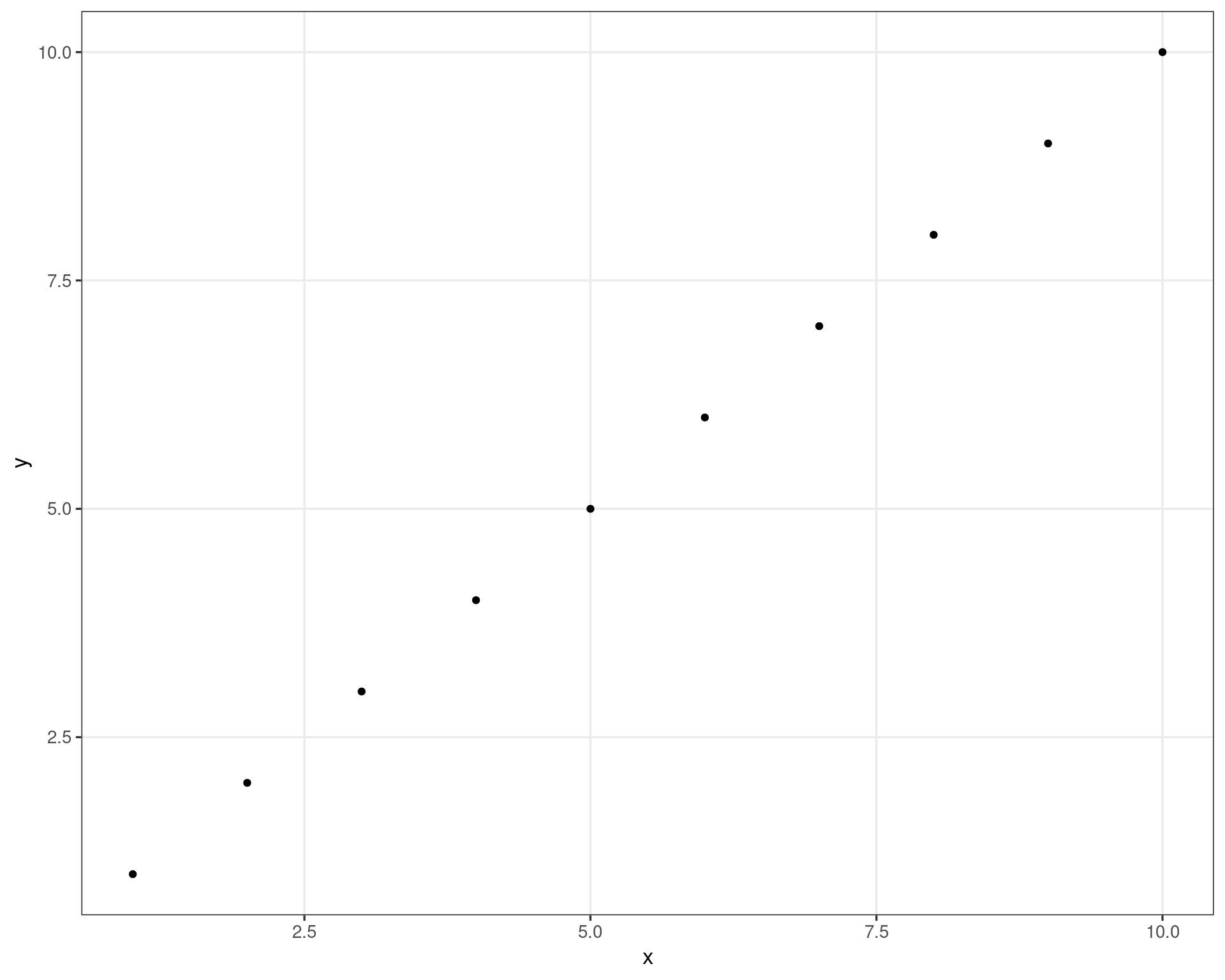
Revisiting the traveling salesperson problem, we saw previously that we can easily perform the necessary calculations outside of ggplot2; avoiding the hassle of defining GeomSalesperson and friends:
ggplot2 is using the same split-apply-combine strategy for each layer, $compute_layer() and $draw_layer() methods call $compute_panel() or $draw_panel() for each class!
GeomComplete$draw_layer#> <ggproto method>#> <Wrapper function>#> function (...) #> draw_layer(..., self = self)#> #> <Inner function (f)>#> function (self, data, params, layout, coord) #> {#> if (empty(data)) {#> n <- if (is.factor(data$PANEL)) #> nlevels(data$PANEL)#> else 1L#> return(rep(list(zeroGrob()), n))#> }#> params <- params[intersect(names(params), self$parameters())]#> if (nlevels(as.factor(data$PANEL)) > 1L) {#> data_panels <- split(data, data$PANEL)#> }#> else {#> data_panels <- list(data)#> }#> lapply(data_panels, function(data) {#> if (empty(data)) #> return(zeroGrob())#> panel_params <- layout$panel_params[[data$PANEL[1]]]#> inject(self$draw_panel(data, panel_params, coord, !!!params))#> })#> }
ggplot2:::CoordCartesian$transform#> <ggproto method>#> <Wrapper function>#> function (...) #> transform(...)#> #> <Inner function (f)>#> function (data, panel_params) #> {#> data <- transform_position(data, panel_params$x$rescale, #> panel_params$y$rescale)#> transform_position(data, squish_infinite, squish_infinite)#> }
# Can debug interactively with {ggtrace}# to learn about `panel_params$x/y$rescale()`ggtrace::ggdebugonce(ggplot2:::CoordCartesian$transform)panel_params$x$rescale#> <ggproto method>#> <Wrapper function>#> function (...) #> rescale(..., self = self)#> #> <Inner function (f)>#> function (self, x) #> {#> self$scale$rescale(x, self$limits, self$continuous_range)#> }
Avoiding grid with $setup_data()
The $setup_data() method allows Geoms to “intercept” the layer’s data before the $draw_*() hierarchy
This is of limited use, mainly for “row-wise” operations
We can attempt to implement GeomComplete with this strategy, however we will quickly run into problems
GeomComplete <-ggproto("GeomComplete", GeomSegment,required_aes =c("x", "y"),setup_data =function(data, params) { data_expanded <- data[rep(1:nrow(data), each =nrow(data)), ] data_expanded$xend <-rep(data$x, times =nrow(data)) data_expanded$yend <-rep(data$y, times =nrow(data)) data_expanded })
# Need to be careful: `$setup_data()`# is not split-apply-combine'ddf_circles <-data.frame(x =cos(seq(0, 2*pi, length.out =16))[-16],y =sin(seq(0, 2*pi, length.out =16))[-16],class =rep(c("a", "b", "c"), times =5))ggplot(df_circles) +geom_complete(aes(x, y, color = class)) +geom_point_new(aes(x, y, fill = class), size =3) +coord_fixed()
Another way to avoid grid
We can use existing $draw_layer(), $draw_panel(), and $draw_group() methods in new Geom objects.
This allows a much easier (and less error-prone) implementation of GeomComplete
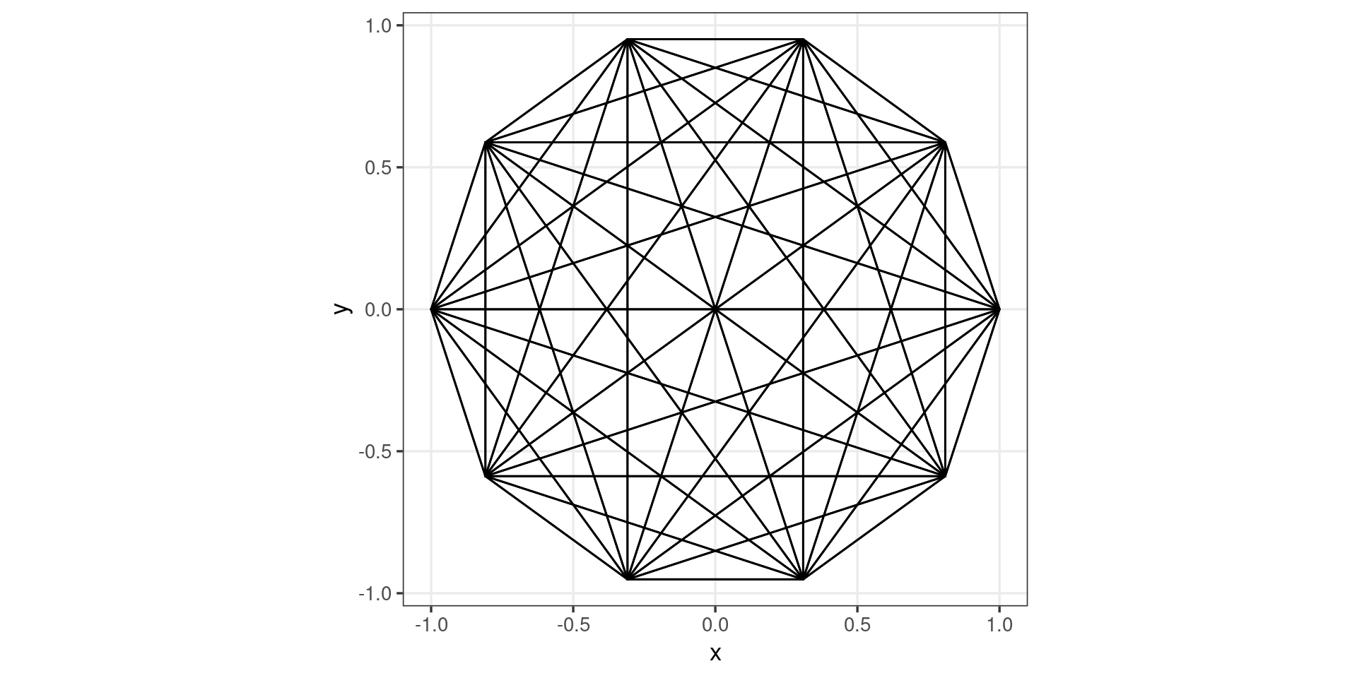
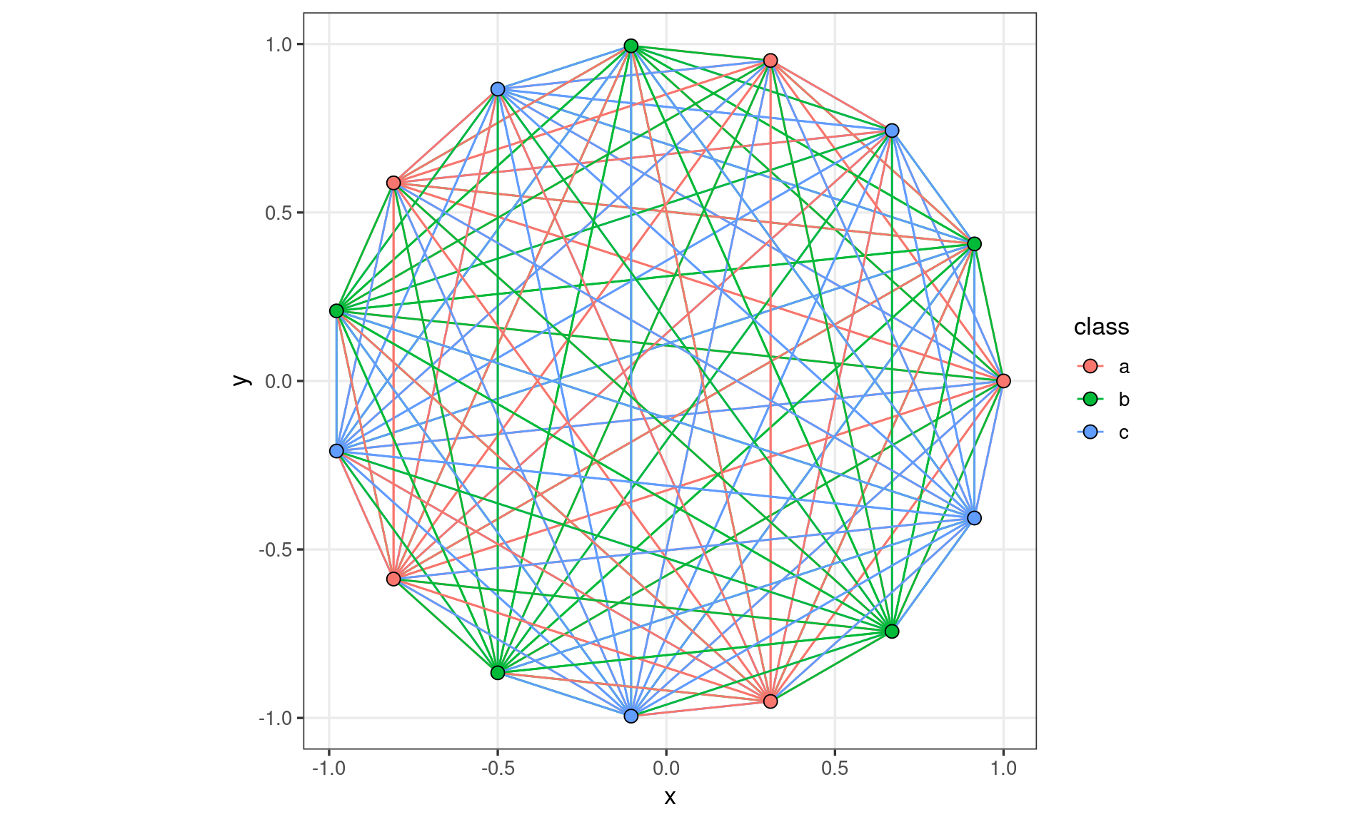
GeomComplete <-ggproto("GeomComplete", Geom,required_aes =c("x", "y"),default_aes =aes(colour ="black",linewidth =0.5,linetype =1,alpha =NA ),non_missing_aes =c("linetype", "linewidth", "shape"), draw_group =function(data, panel_params, coord, ...) { data_expanded <- data[rep(1:nrow(data), each =nrow(data)), ] data_expanded$xend <-rep(data$x, times =nrow(data)) data_expanded$yend <-rep(data$y, times =nrow(data))# hand group-level data off to GeomSegment$draw_panel() GeomSegment$draw_panel(data_expanded, panel_params, coord, ...) },draw_key = draw_key_path)
df_circles <-data.frame(x =cos(seq(0, 2*pi, length.out =16))[-16],y =sin(seq(0, 2*pi, length.out =16))[-16],class =rep(c("a", "b", "c"), times =5))ggplot(df_circles) +geom_complete(aes(x, y, color = class)) +geom_point_new(aes(x, y, fill = class), size =3) +coord_fixed()
Other ways to extend ggplot2
Aside from implementing new Geom and Statggproto objects, there are other formal ways to extend ggplot2:
New color palettes for scale_color/fill()
Customized themes
New coordinate systems
New scales
New faceting systems
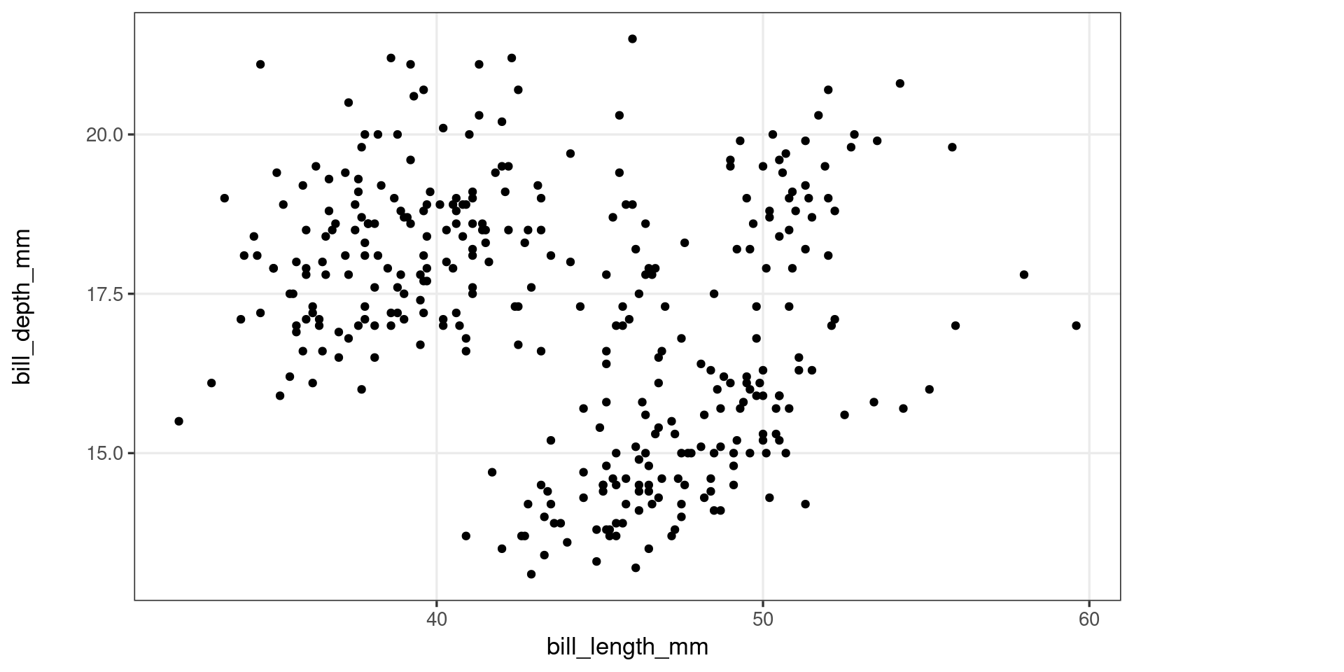
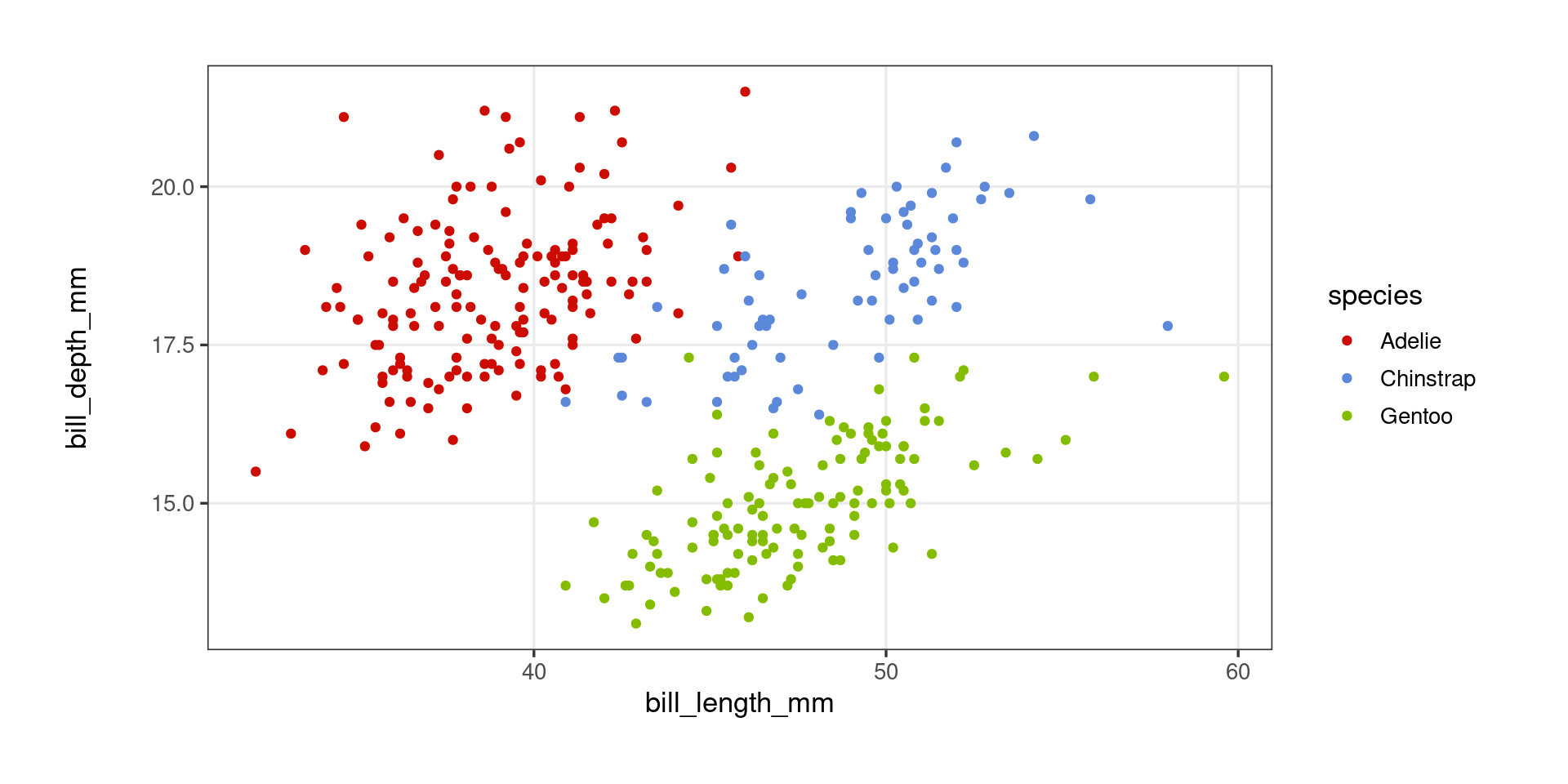
ggplot(penguins, aes(x = bill_length_mm, y = bill_depth_mm, color = species)) +geom_point()
ggplot(penguins, aes(x = bill_length_mm, y = bill_depth_mm, color = species)) +geom_point() + ggsci::scale_color_startrek()
ggplot(penguins, aes(x = bill_length_mm, y = bill_depth_mm)) +geom_point() + hrbrthemes::theme_ipsum_rc()