Univariate histogram HDR estimator — method_histogram

Function used to specify univariate histogram density estimator for get_hdr_1d() and layer functions (e.g. geom_hdr_rug()).

Usage

method_histogram_1d(bins = NULL)

Arguments

bins: Number of bins. Defaults to normal reference rule (Scott, pg 59).

Details

For more details on the use and implementation of the method_*_1d() functions, see vignette("method", "ggdensity").

References

Scott, David W. Multivariate Density Estimation (2e), Wiley.

Examples

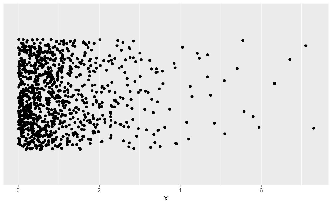
# Histogram estimators can be useful when data has boundary constraints
df <- data.frame(x = rexp(1e3))

# Strip chart to visualize 1-d data
p <- ggplot(df, aes(x)) +
  geom_jitter(aes(y = 0), width = 0, height = 2) +
  scale_y_continuous(name = NULL, breaks = NULL) +
  coord_cartesian(ylim = c(-3, 3))

p


p + geom_hdr_rug(method = method_histogram_1d())


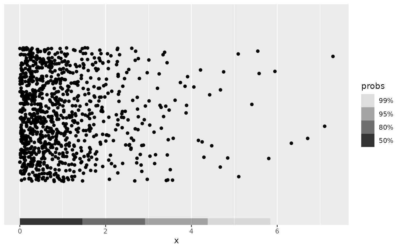
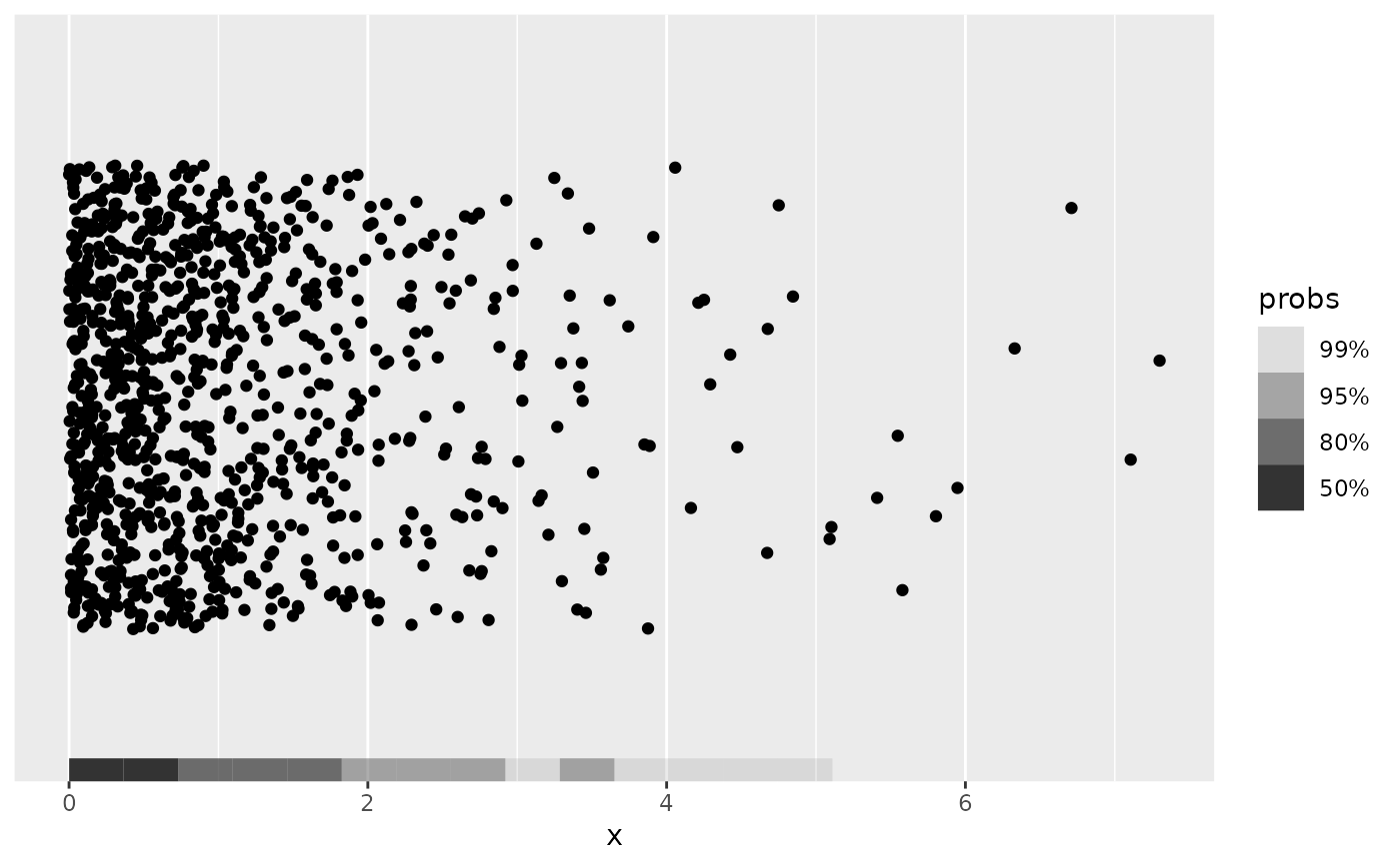# The resolution of the histogram estimator can be set via `bins`
p + geom_hdr_rug(method = method_histogram_1d(bins = 5))


# Can also be used with `get_hdr_1d()` for numerical summary of HDRs
res <- get_hdr_1d(df$x, method = method_histogram_1d())
str(res)
#> List of 3
#>  $ df_est:'data.frame':	20 obs. of  4 variables:
#>   ..$ x               : num [1:20] 0.183 0.548 0.913 1.278 1.643 ...
#>   ..$ fhat            : num [1:20] 0.3003 0.2132 0.1682 0.0921 0.0691 ...
#>   ..$ fhat_discretized: num [1:20] 0.3003 0.2132 0.1682 0.0921 0.0691 ...
#>   ..$ hdr             : num [1:20] 0.5 0.5 0.8 0.8 0.8 0.95 0.95 0.95 0.99 0.95 ...
#>  $ breaks: Named num [1:5] 0.004 0.016 0.0691 0.2132 Inf
#>   ..- attr(*, "names")= chr [1:5] "99%" "95%" "80%" "50%" ...
#>  $ data  :'data.frame':	1000 obs. of  2 variables:
#>   ..$ x             : num [1:1000] 2.073 1.628 3.268 1.354 0.224 ...
#>   ..$ hdr_membership: num [1:1000] 0.95 0.8 0.99 0.8 0.5 0.5 0.5 0.5 0.95 0.5 ...